 Nima Leclerc
Explained · 07 · Preprint · submitted to npj Quantum Information
Beyond sensitivity: an error budget for quantum sensors
One simulation that tells you not just how sensitive a sensor is, but what is limiting its accuracy and robustness.
The problem
Quantum sensors are usually advertised with one number, their sensitivity: the smallest field they can resolve per unit of measurement time. But a navigation system needs accuracy, the measured value being right and not just precise, and a heart monitor used outside a shielded room needs robustness against a drifting background. A sensor tuned for one can fall short on the others, and today the trade-offs are mostly settled by expert judgment and bench trial and error.
The idea
Precision instruments such as gravitational-wave detectors and atomic clocks keep an error budget, a ledger of how much each noise source contributes. Quantum sensors have been harder to budget, because the error sources interact inside one nonlinear measurement cycle, so you cannot just add them up.
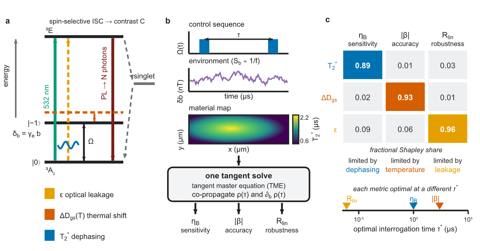
We built a framework that treats the sensor as an open quantum system and solves its dynamics once. From that single solve it computes all three metrics. To split each one among the physical causes, it uses Shapley values, a fair-division method from game theory that is also used to explain machine-learning models, and that handles interacting contributors properly.
What it found for diamond NV sensors
The culprit changes with the metric.
- Sensitivity is limited mainly by spin dephasing.
- Accuracy is limited by the temperature shift of the ground-state splitting.
- Robustness is limited by optical leakage.
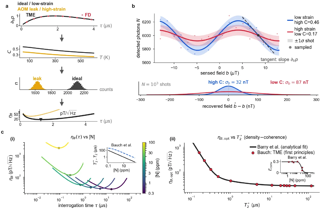
The consequence is striking. At the same sensitivity, the error in the recovered field can range from 8 to 1500 nanotesla, so tuning for sensitivity alone could miss an accuracy target by two orders of magnitude.
A second sensor, a real heartbeat
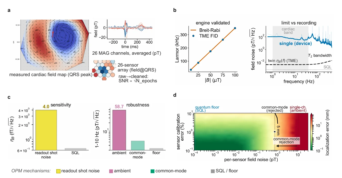
To test that the approach is not specific to diamond, we applied it to a 26-sensor array of cesium optical magnetometers recording a human magnetocardiogram, the magnetic signal of the heart. A model grounded in the recording reproduces the expected Larmor behavior, and the resulting budgets show where the design margin lies: in rejecting ambient noise rather than in the atomic limit.
Why this matters: a digital twin
Because the model is built from the device physics, it works as a digital twin: you can ask it what would improve if you fixed one limiter, before building anything. That is how sensor design can move from iteration to specification.
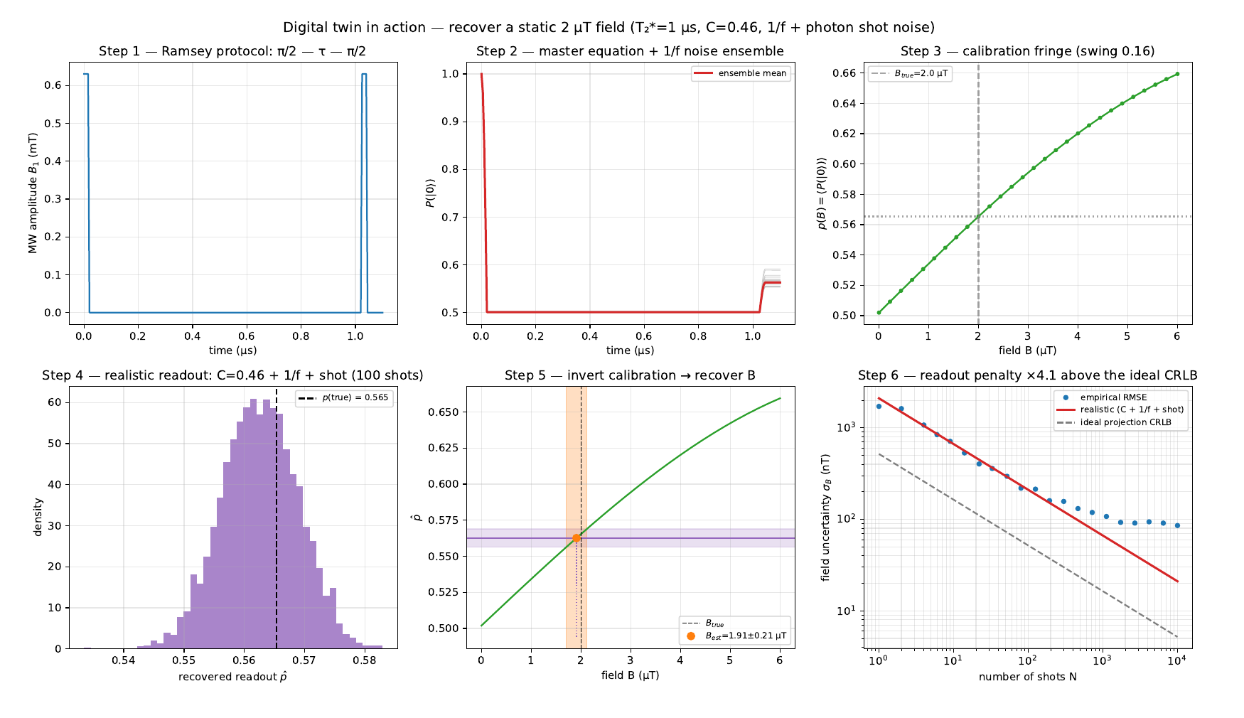
The supplementary example below follows the whole chain once: simulate the pulse sequence, draw noisy photon counts, and invert the calibration to recover a known field. It makes visible exactly which imperfections separate a real device from the quantum limit.
Caveats
The literature comparisons use assumed collection factors, so they are consistency checks, not parameter-free predictions, and the manuscript is a preprint still under review.